

Mesh#
Meshes are required to discretise the geometrical domain of the simulation. As FESTIM is not a meshing tool, the meshing capabilities are limited to simple 1D meshes.
1D meshes#
The easiest way to define a 1D mesh in FESTIM is to define it from a list of vertices (see festim.MeshFromVertices):
mesh = MeshFromVertices([0, 1, 2, 4, 5, 10])
For bigger meshes, use the numpy library to generate an array of vertices.
import numpy as np

mesh = MeshFromVertices(np.linspace(0, 10, num=1000))
Numpy arrays can be combined to have local refinements:
import numpy as np

vertices = np.concatenate(
    [
        np.linspace(0, 1e-6, num=100),  # 99 cells between 0 and 1 micron
        np.linspace(1e-6, 1e-4, num=100),  # 99 cells between 1 micron and 0.1 mm
        np.linspace(1e-4, 1e-2, num=10)  # 9 cells between 0.1 mm and 1 cm
    ]
)
mesh = MeshFromVertices(vertices)
Meshes from XDMF#
More complex meshes can be read from XDMF files (see festim.MeshFromXDMF):
mesh = MeshFromXDMF(volume_file="volume_file.xdmf", boundary_file="boundary_file.xdmf")
Succesfully load mesh with 200 cells
The recommended workflow is to mesh your geometry with your favourite meshing software (SALOME, gmsh…) and convert the produced mesh with meshio.
GMSH example#
The DOLFINx tutorial gives an example of mesh generation with gmsh, and additionally the GMSH reference manual can be accessed here
The following is a workflow using the python API to make a mesh that can be directly integrated into FESTIM:
Here we will walk through GMSH’s usage when creating a monoblock subsection consisting of tungsten surrounding a tube of CuCrZr
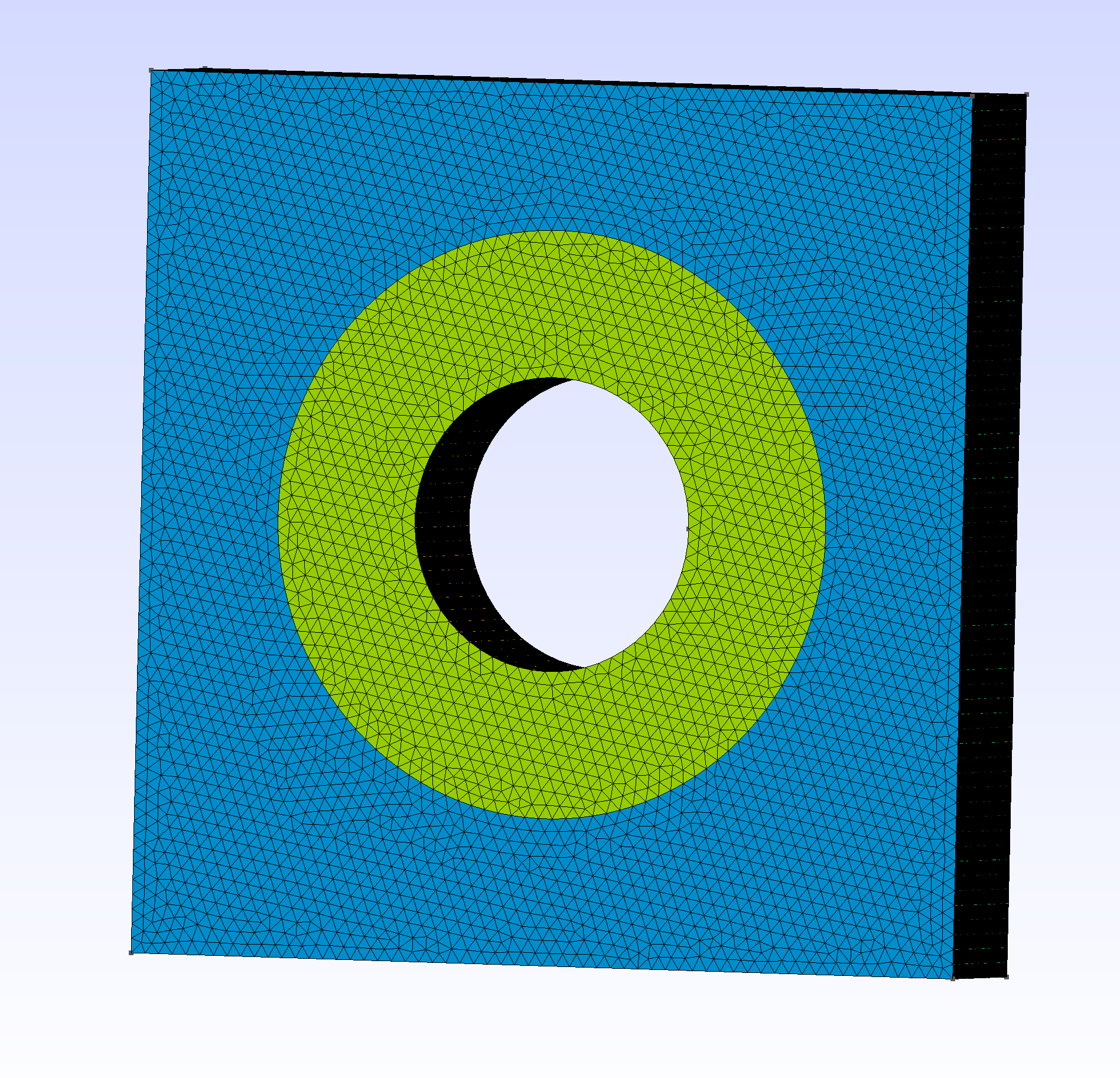
Meshing the geometry with GMSH#
GMSH can be installed via the following link.
To use the Python API, gmsh will need to be pip installed using
pip install gmsh
Now, GMSH must be imported and initialised.
import gmsh as gmsh

gmsh.initialize()
gmsh.model.add("mesh")
We can set the size of our mesh using:
lc = 1e-3
Models in GMSH consist of a series of:
Points
Lines
Wires / Curve Loops - whether we use curve loops or wires depends on whether we use the .occ or .geo geometry kernels. .occ allows for direct construction of more complex features such as cylinders, whereas using .geo requires explicit user definition of all the points, surfaces and volumes that would make up the cylinder.
Surfaces
Surface Loops
Volumes
We will begin by defining the points of our square of tungsten.
p1 = gmsh.model.occ.addPoint(-15e-3, 15e-3, 0, lc)
p2 = gmsh.model.occ.addPoint(-15e-3, -15e-3, 0, lc)
p3 = gmsh.model.occ.addPoint(15e-3, 15e-3, 0, lc)
p4 = gmsh.model.occ.addPoint(15e-3, -15e-3, 0, lc)
These points can then be joined together using lines. It is important that we pay close attention to the direction that these lines are going.
line_1_2 = gmsh.model.occ.addLine(p1, p2)
line_1_3 = gmsh.model.occ.addLine(p1, p3)
line_2_4 = gmsh.model.occ.addLine(p2, p4)
line_3_4 = gmsh.model.occ.addLine(p3, p4)
These are then used to create curve loops or wires. Wires and curve loops must be closed loops, and the list of lines must flow in the correct direction so as to form a complete loop.
base_loop = gmsh.model.occ.addWire([line_1_2, line_2_4, -line_3_4, -line_1_3])
We can also define the inner and outer circles and loops for the CuCrZr tube.
inner_circle = gmsh.model.occ.addCircle(0,0,0,5e-3)
outer_circle = gmsh.model.occ.addCircle(0,0,0,10e-3)

inner_circle_loop = gmsh.model.occ.addWire([inner_circle])
outer_circle_loop = gmsh.model.occ.addWire([outer_circle])
Surfaces are defined using loops, where the first loop in the list denotes the outer borders of the surface, and any others define holes within the surface. Here base_surface is our tungsten layer, and so it consists of our base rectangle curve loop, with a hole defined by the outer CuCrZr loop.
base_surface = gmsh.model.occ.addPlaneSurface([base_loop, outer_circle_loop])
cylinder_surface = gmsh.model.occ.addPlaneSurface([outer_circle_loop, inner_circle_loop])
While we could then define another surface above the first and join them together, it is often easier to just perform an extrusion of the surfaces. Here we stretch both the tungsten and CuCrZr surfaces by 5e-3 in the z-direction, and 0 in the x and y.
outer_layer_extrusion = gmsh.model.occ.extrude(
    [(2, base_surface)], 0, 0, 5e-3, numElements=[100]
)
interface_layer_extrusion = gmsh.model.occ.extrude(
    [(2, cylinder_surface)], 0, 0, 5e-3, numElements=[100]
)
Upon performing the extrusion, GMSH will define any necessary surfaces and volumes for us. However, this means that the surface of the outer cylinder will have been defined twice. Therefore it is necessary to remove any duplicate elements via
remove_overlap = gmsh.model.occ.remove_all_duplicates()
It is important that all points in our model are defined using the same characteristic length. Therefore we need to define a couple of points across the mesh to have the same lc. Here we have used points on the inner and outer tube perimeters, on both the front and back of the mesh:
inner_front_perimiter_point = gmsh.model.occ.addPoint(5e-3, 0, 5e-3, lc)
inner_back_perimiter_point = gmsh.model.occ.addPoint(5e-3, 0, 0, lc)

outer_front_perimiter_point = gmsh.model.occ.addPoint(10e-3, 0, 5e-3, lc)
outer_back_perimiter_point = gmsh.model.occ.addPoint(10e-3, 0, 0, lc)
The model can then be synchronized:
gmsh.model.occ.synchronize()
At any point, the GMSH GUI can be opened by running the line
gmsh.fltk.run()
after synchronizing the model. Running this command at this stage will open the GUI, displaying something that looks like this:
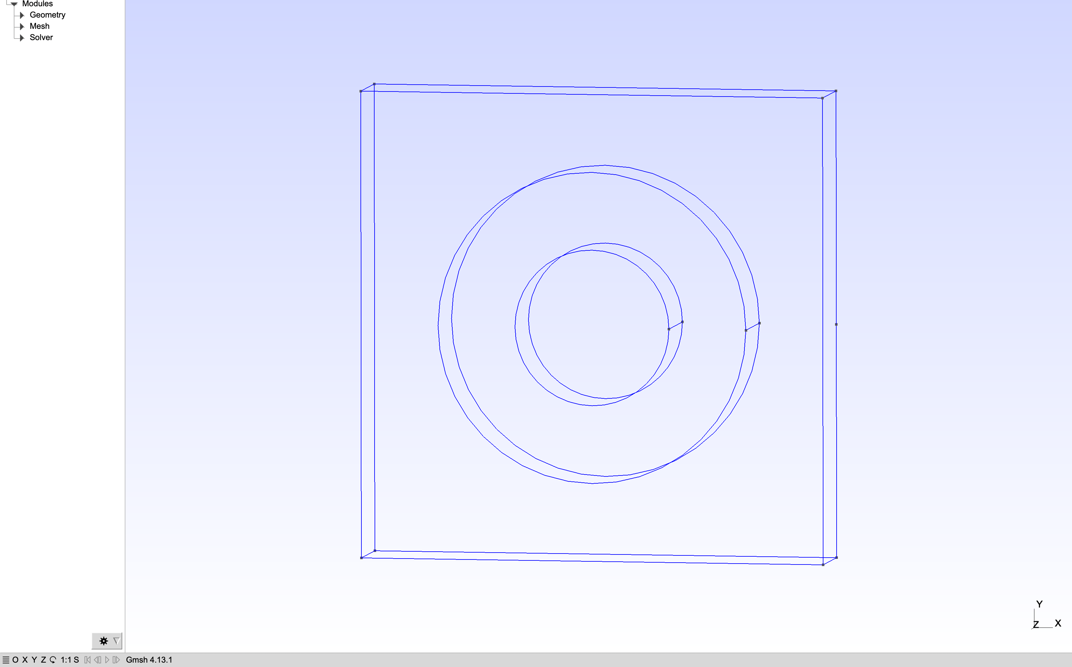
To be used with FESTIM, it is necessary for us to define surface and volume markers.
If the element has been defined explicitly, this is as easy as doing the following:
id_number = 1
gmsh.model.addPhysicalGroup(2, [base_surface, cylinder_surface], id_number, name="surface")
where the 2 indicates that this is a 2nd dimension element, and we have listed the surfaces that we would like to assign with this ID number.
However, as we generated the surfaces using an extrusion, it can be complicated to keep track of which element corresponds to what. GMSH assigns the surface labels cyclically when performing the extrusion, so these element IDs could be directly extracted using code. However, it may be more straightforward and intuitive to open the GUI as before and analyze the surfaces manually.
After opening the GUI, again after synchronising and using gmsh.fltk.run(), go into ‘Tools’ then ‘Options’, and ensure that ‘Surfaces’ is checked under ‘Geometry’. This will make the surfaces are visible and selectable in the visualisation.
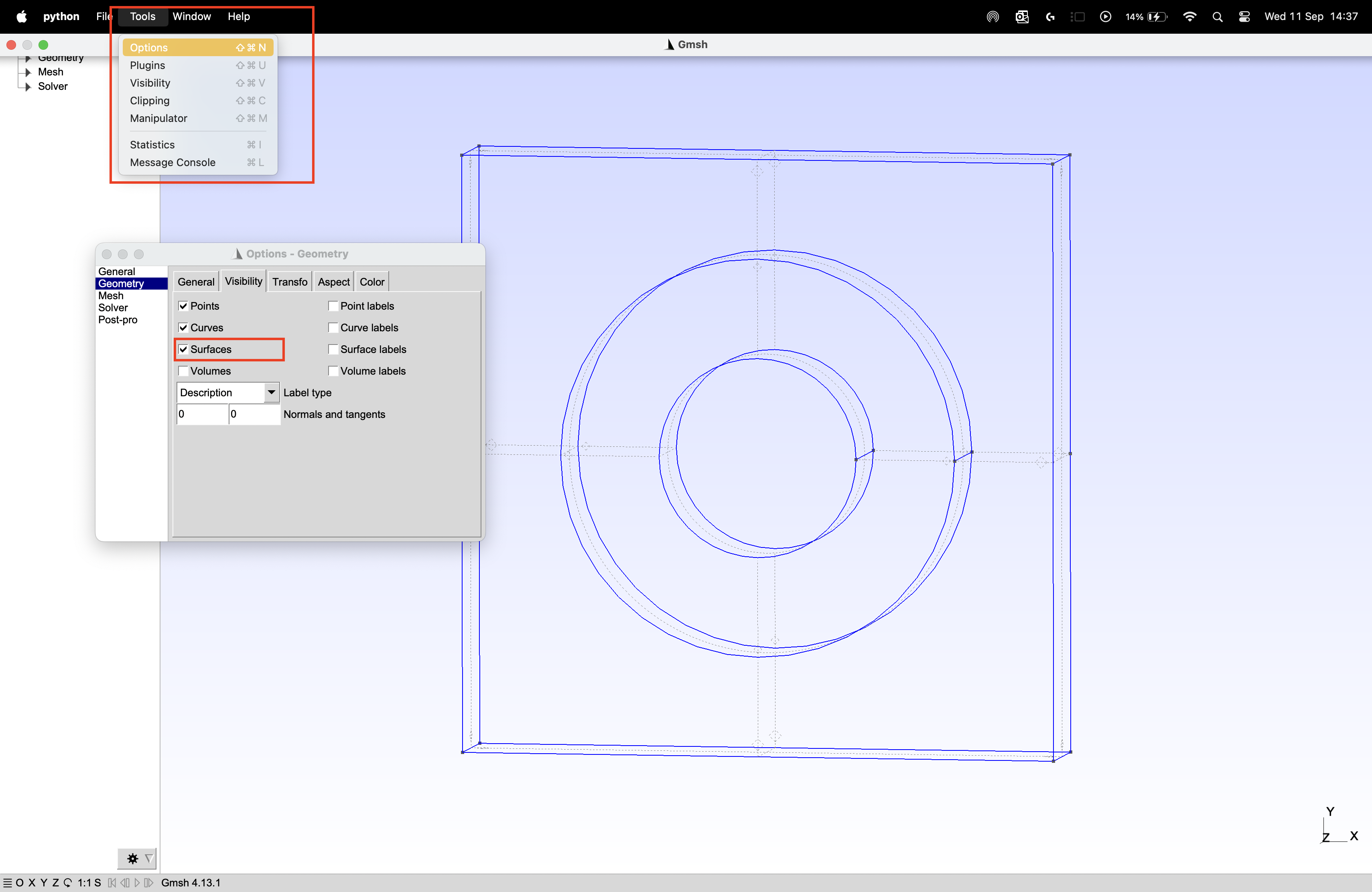
We can then hover our mouse over each surface to see its information. For example, we can see that the front tungsten surface is defined as Plane 7, and borders the volume 1.
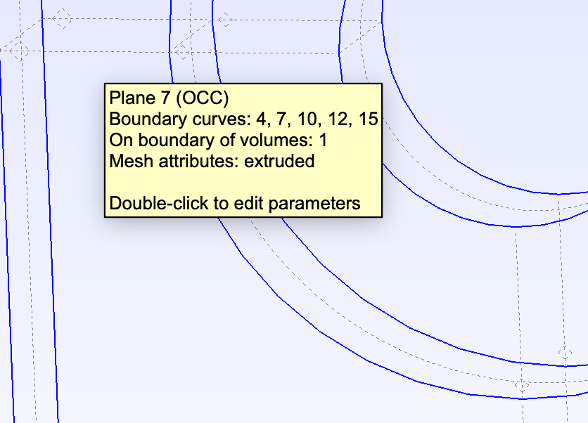
We can now look at each surface and interface and assign the necessary IDs.
front_id = 1
back_id = 2
left_id = 3
right_id = 4
top_id = 5
bottom_id = 6
outer_cylinder_surface_id = 7
inner_cylinder_surface_id = 8

tungsten_id = 1
cucrzr_id = 2

gmsh.model.addPhysicalGroup(2, [7, 10], front_id, name="front")
gmsh.model.addPhysicalGroup(2, [6, 9], back_id, name="back")
gmsh.model.addPhysicalGroup(2, [1], left_id, name="left")
gmsh.model.addPhysicalGroup(2, [3], right_id, name="right")
gmsh.model.addPhysicalGroup(2, [4], top_id, name="top")
gmsh.model.addPhysicalGroup(2, [2], bottom_id, name="bottom")
gmsh.model.addPhysicalGroup(
    2, [5], outer_cylinder_surface_id, name="tungsten_cucrzr_interface"
)
gmsh.model.addPhysicalGroup(
    2, [8], inner_cylinder_surface_id, name="cucrzr_coolant_interface"
)

gmsh.model.addPhysicalGroup(3, [1], tungsten_id, name="tungsten")
gmsh.model.addPhysicalGroup(3, [2], cucrzr_id, name="cucrzr")
The model must then be resynchronized before generating the mesh.
gmsh.model.occ.synchronize()

gmsh.model.mesh.generate(3)
The mesh can then be written to a file, and GMSH finalised.
gmsh.write("my_mesh.msh")
gmsh.finalize()
We have now created our mesh!
Converting meshes using meshio#
However, for use in FESTIM, our mesh now has to be converted into XDMF files, and the surfaces and volume IDs extracted.
This can be done using meshio via the following process:
import meshio
import numpy as np

msh = meshio.read("my_mesh.msh")

# Initialize lists to store cells and their corresponding data
triangle_cells_list = []
tetra_cells_list = []
triangle_data_list = []
tetra_data_list = []

# Extract cell data for all types
for cell in msh.cells:
    if cell.type == "triangle":
        triangle_cells_list.append(cell.data)
    elif cell.type == "tetra":
        tetra_cells_list.append(cell.data)

# Extract physical tags
for key, data in msh.cell_data_dict["gmsh:physical"].items():
    if key == "triangle":
        triangle_data_list.append(data)
    elif key == "tetra":
        tetra_data_list.append(data)

# Concatenate all tetrahedral cells and their data
tetra_cells = np.concatenate(tetra_cells_list)
tetra_data = np.concatenate(tetra_data_list)

# Concatenate all triangular cells and their data
triangle_cells = np.concatenate(triangle_cells_list)
triangle_data = np.concatenate(triangle_data_list)

# Create the tetrahedral mesh
tetra_mesh = meshio.Mesh(
    points=msh.points,
    cells=[("tetra", tetra_cells)],
    cell_data={"f": [tetra_data]},
)

# Create the triangular mesh for the surface
triangle_mesh = meshio.Mesh(
    points=msh.points,
    cells=[("triangle", triangle_cells)],
    cell_data={"f": [triangle_data]},
)

# Write the mesh files
meshio.write("volume_mesh.xdmf", tetra_mesh)
meshio.write("surface_mesh.xdmf", triangle_mesh)
Using the mesh in FESTIM#
A FESTIM simulation can then be run:
import festim as F

model = F.Simulation()

model.mesh = F.MeshFromXDMF(volume_file ="volume_mesh.xdmf", boundary_file = "surface_mesh.xdmf")

model.materials = [F.Material(id=1, D_0=1, E_D=0),
                    F.Material(id=2, D_0=5, E_D=0)]

model.T = F.Temperature(800)

model.boundary_conditions = [F.DirichletBC(surfaces = [top_id], value = 1, field = 0),
                                F.DirichletBC(surfaces = [inner_cylinder_surface_id], value = 0, field = 0)]

model.exports = [F.XDMFExport("solute")]

model.settings = F.Settings(
    absolute_tolerance=1e-10,
    relative_tolerance=1e-10,
    transient=False,
)

model.initialise()
model.run()
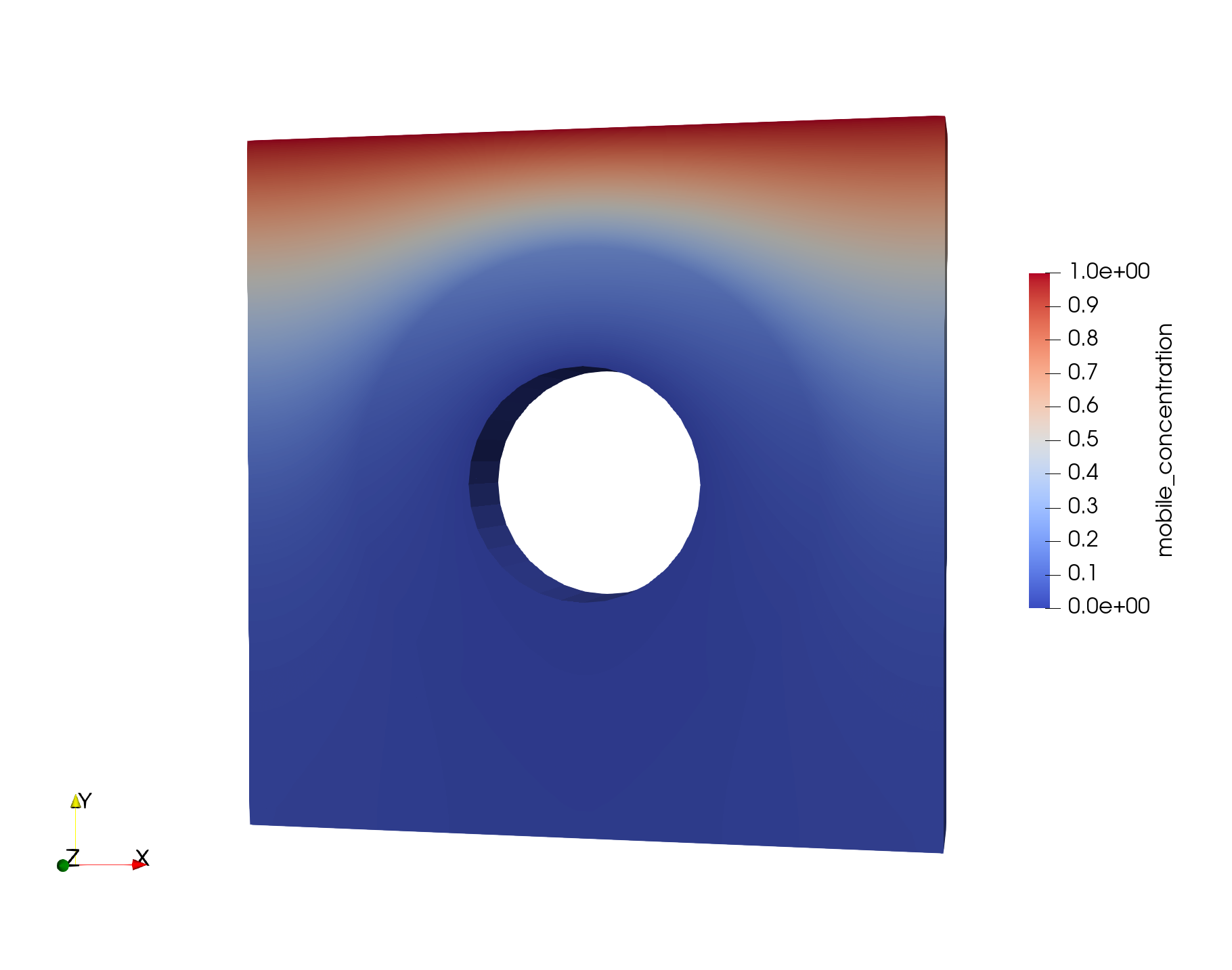
This produces the following visualisation in Paraview:
SALOME example#
This is a step-by-step guide to meshing with SALOME 9.12.0.
Building the geometry in SALOME#
Open SALOME and create a new study.
Activate the Geometry module
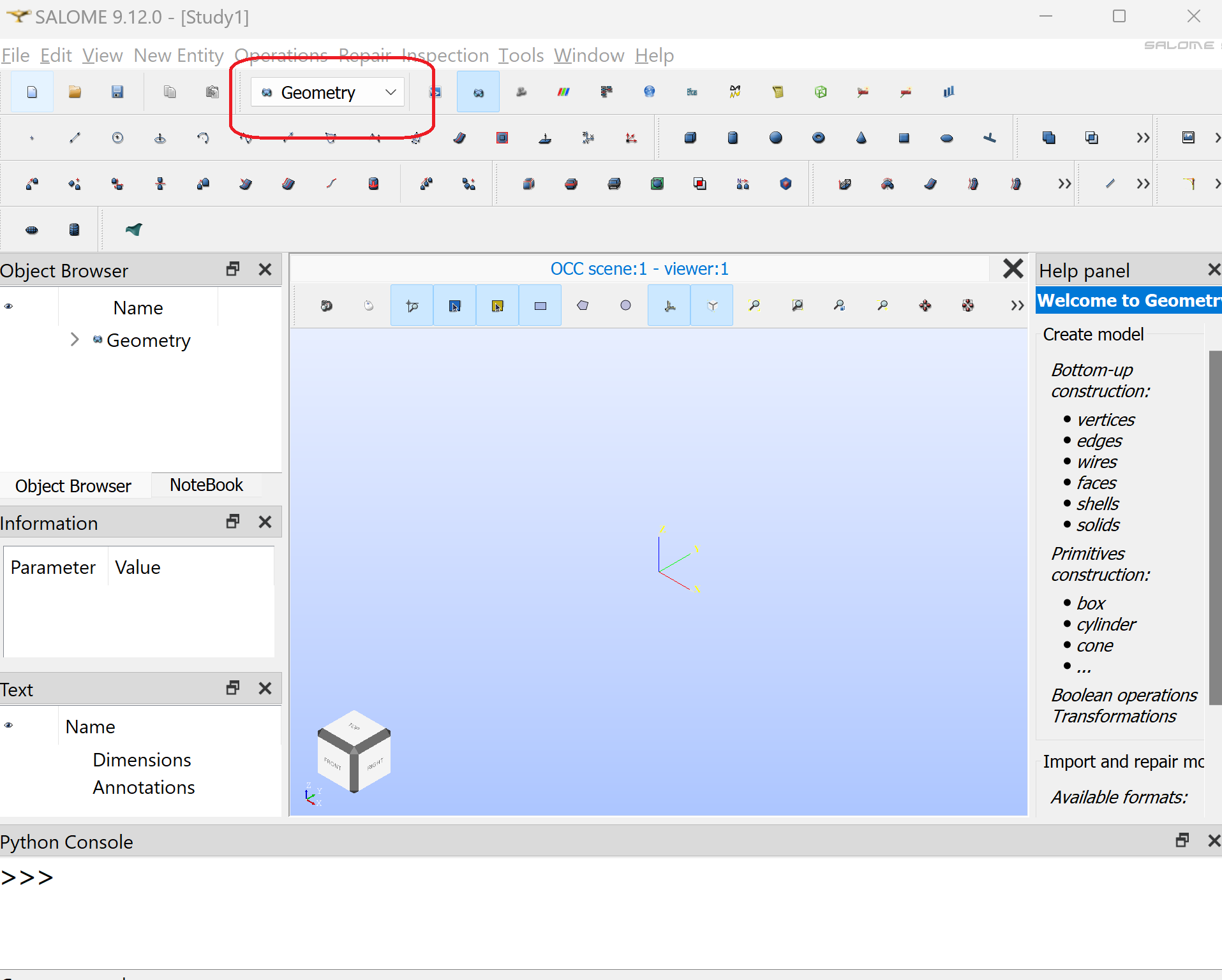
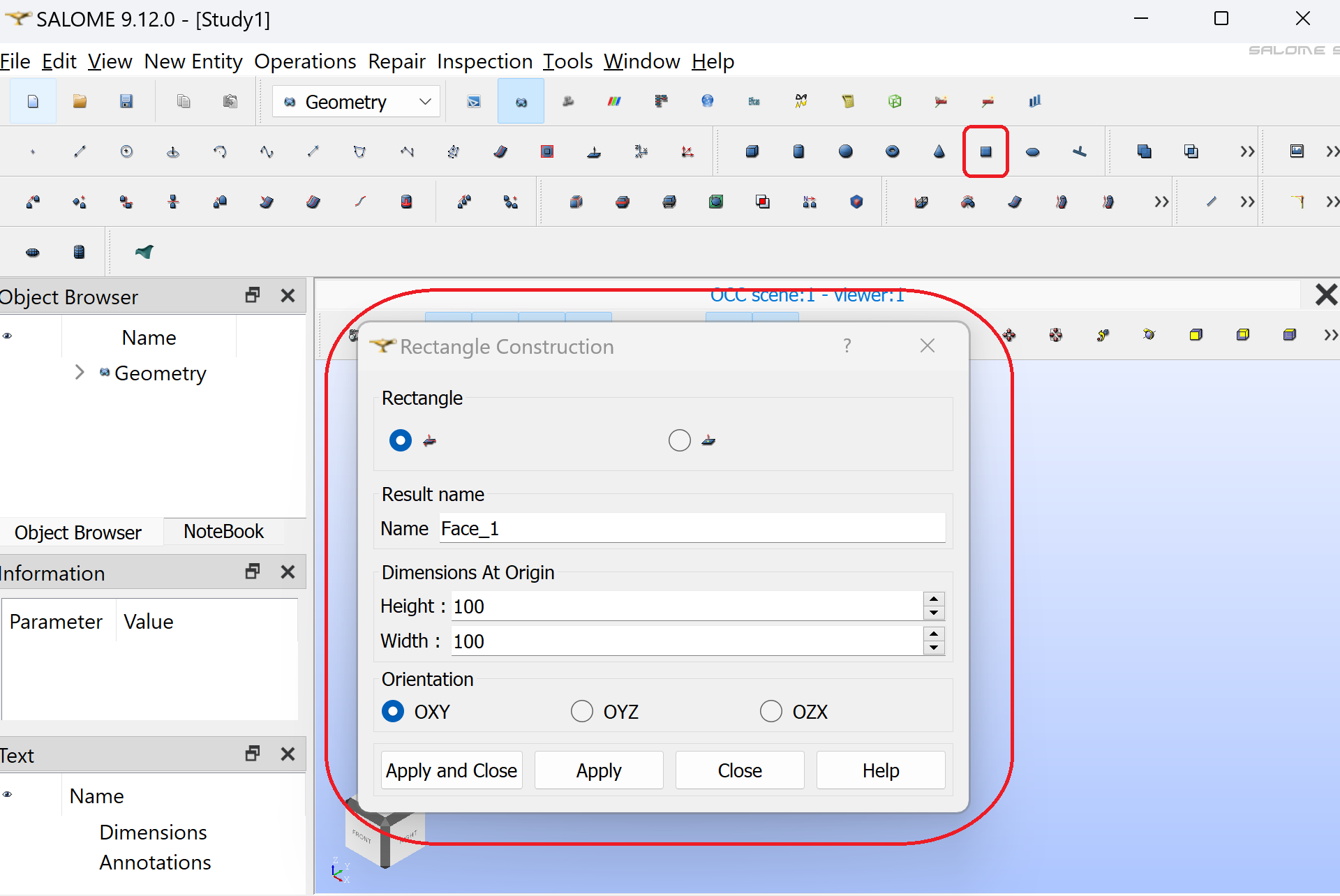
Create a first square by clicking “Create rectangular face”. Keep the default parameters. Click “Apply and Close”
Repeat the operation to create a second square
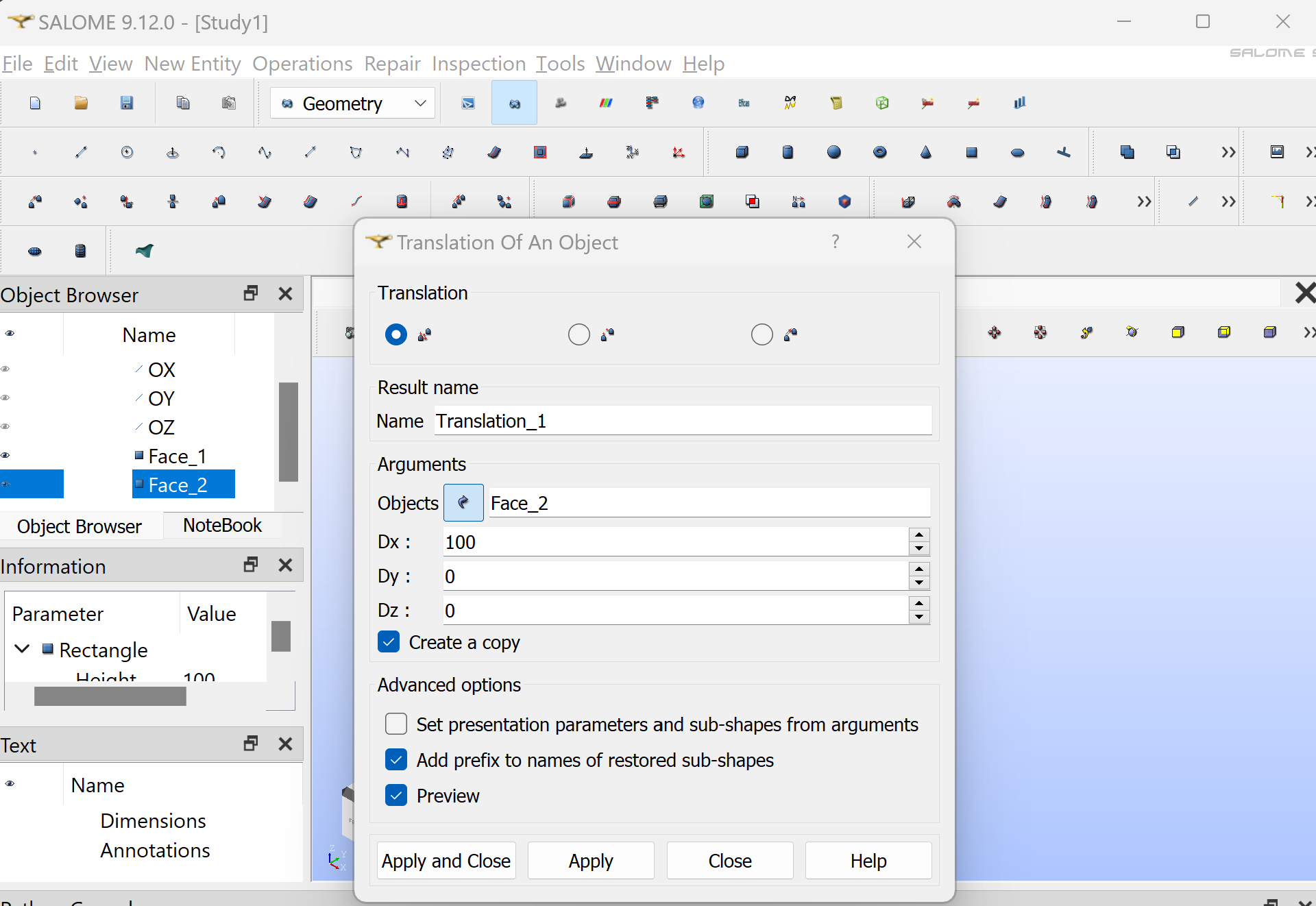
Translate the second square by clicking “Operations/Transformation/Translation”
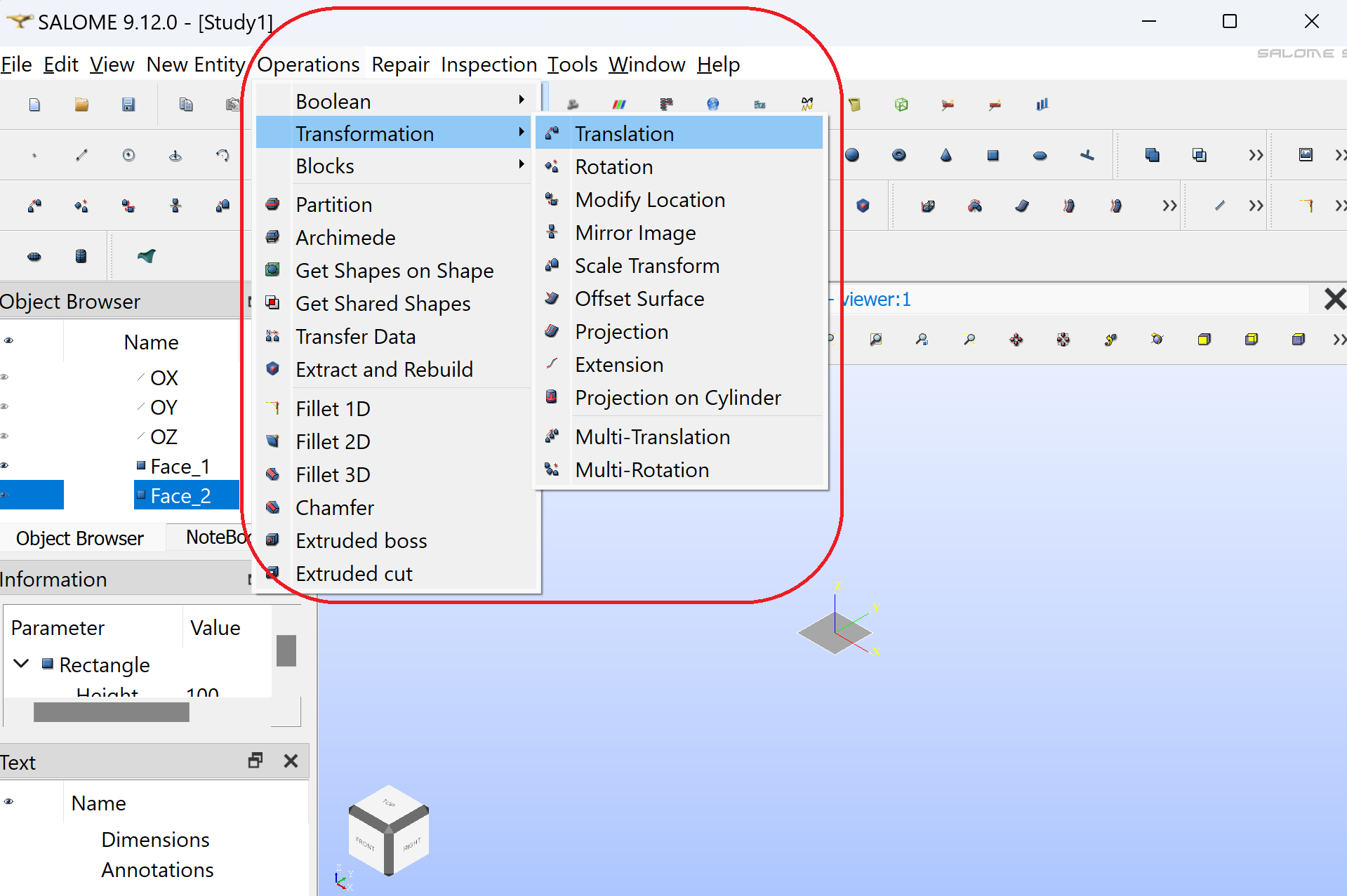
Make sure Face 2 is selected. Enter 100 for the Dx value. Click “Apply and Close”
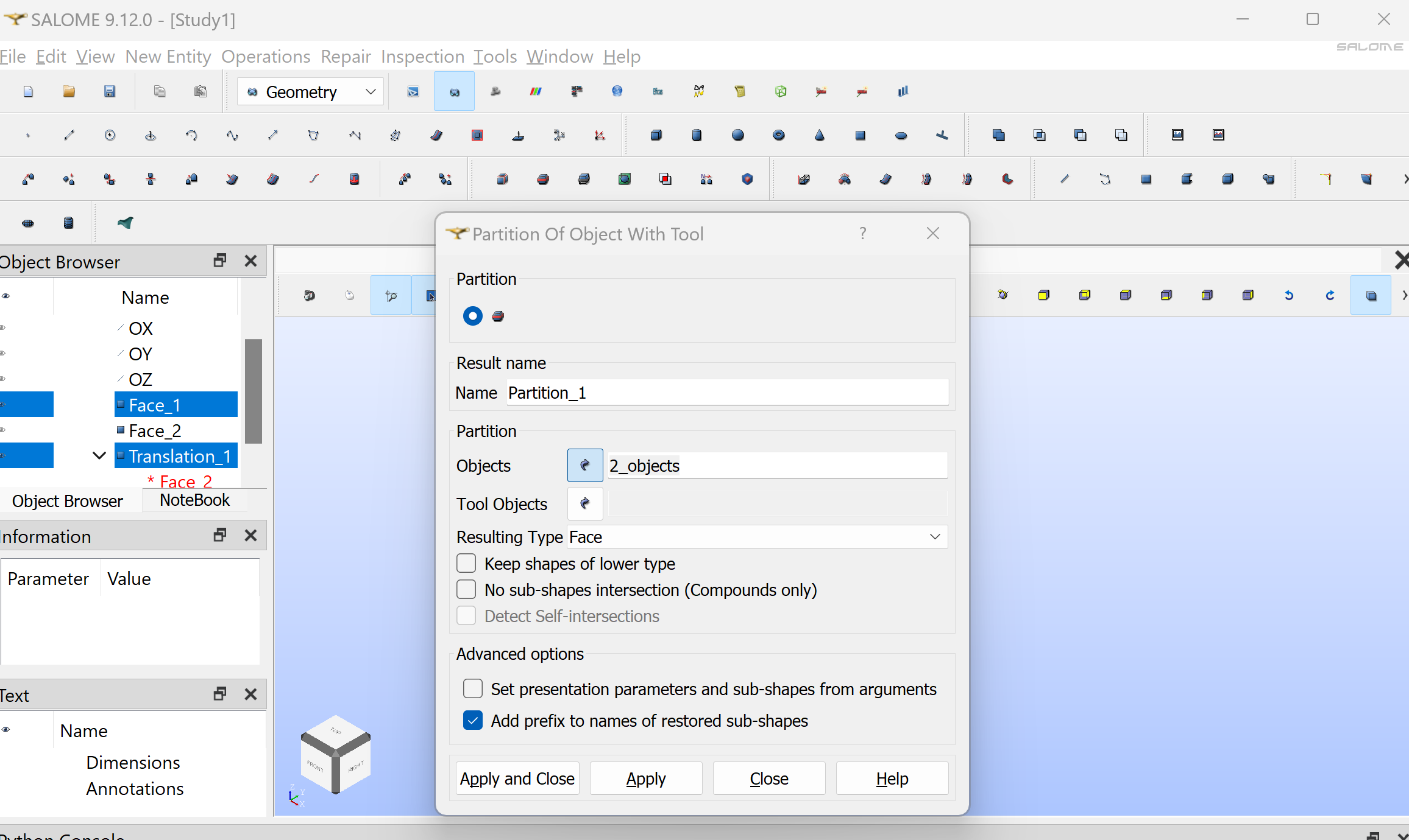
Create a compound by clicking “New Entity/Build/Compound” make sure Face_1 and Translation_1 are selected then click “Apply and Close”.
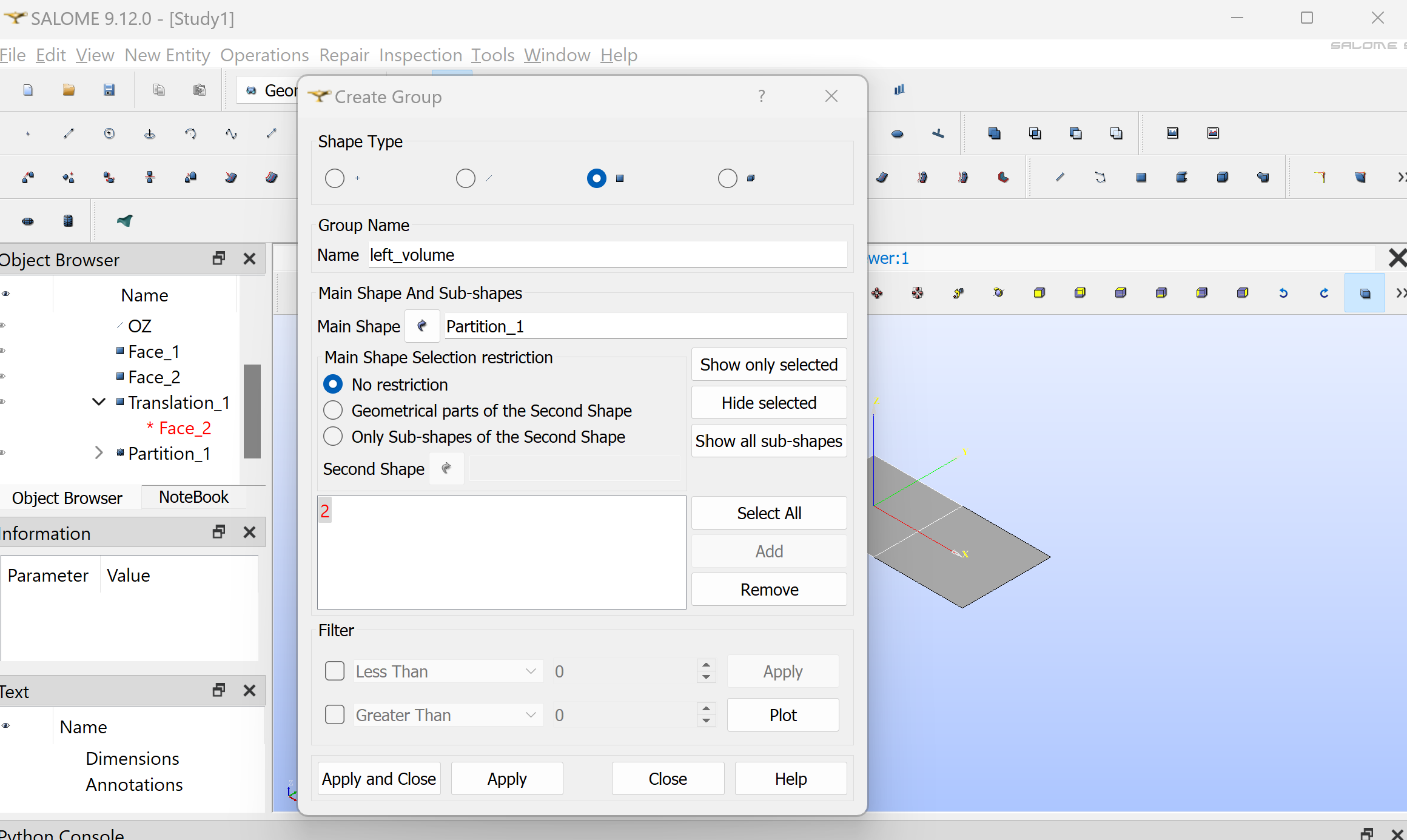
8. Create a group “New Entity/Group/Create group”. In Shape Type, select the 2D surface. Name the group “left_volume”. Make sure Compound_1 is selected. Click on the left square and click “Add” (2 should appear in the white window). Click “Apply and Close”.
Repeat the operation to create a group “right_volume” with the right square (12 should appear in the white window).
Create another group “left_boundary” but this time in Shape Type select the 1D curve. Click on the left edge of the left square and click “Add”. Click “Apply and Close”.
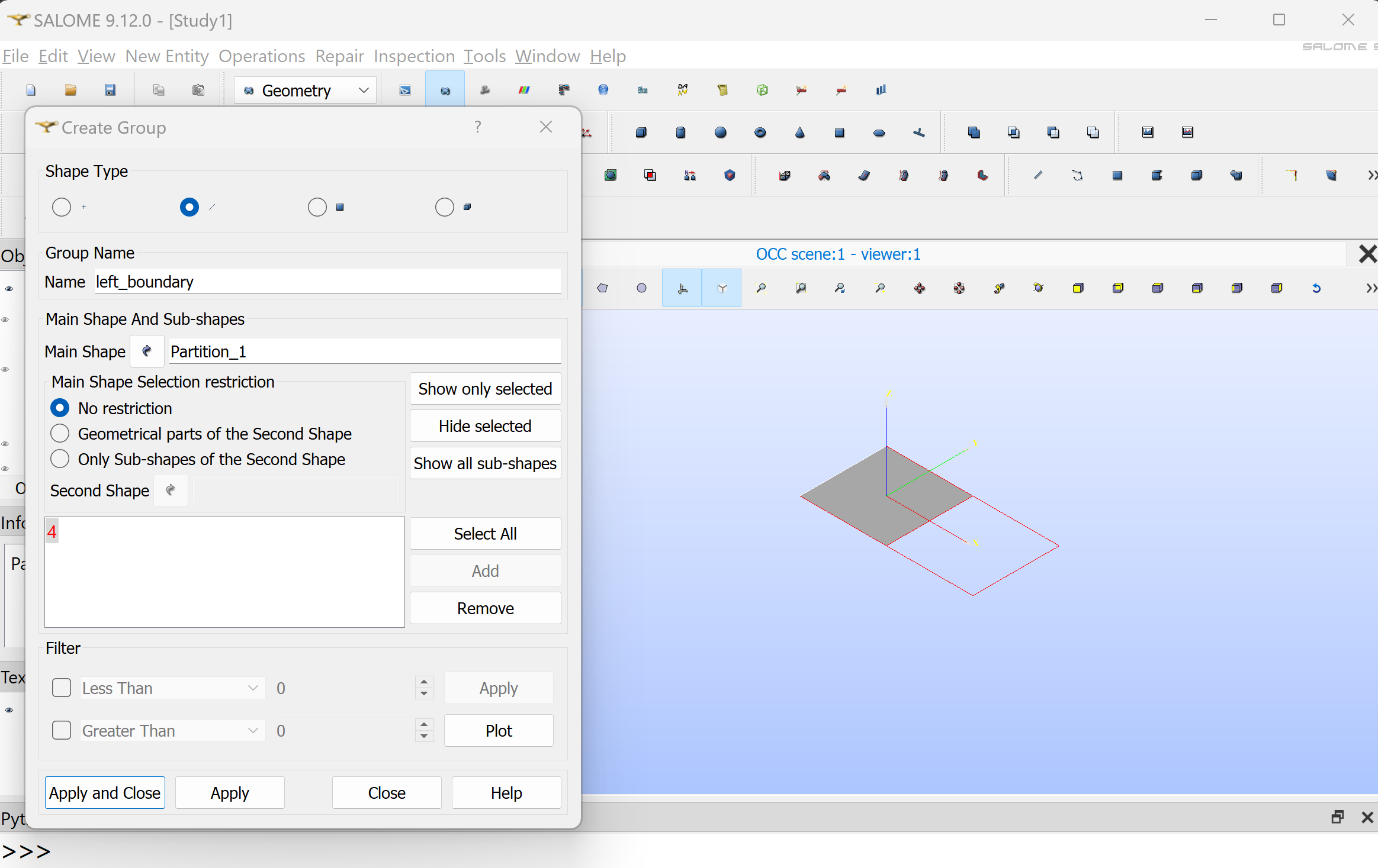
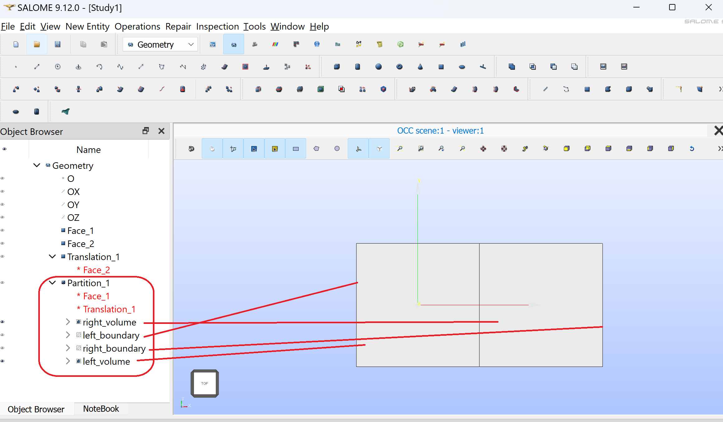
Repeat the operation to create a group “right_boundary” with the right edge of the right square. Your study should look like:
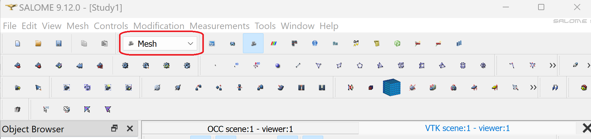
Click on “Mesh” to activate the mesh module.
Create a mesh by clicking “Mesh/Create Mesh”.
Make sure Compound_1 is selected in “Geometry”. Under the 2D tab, select “NETGEN 1D-2D” as algorithm.
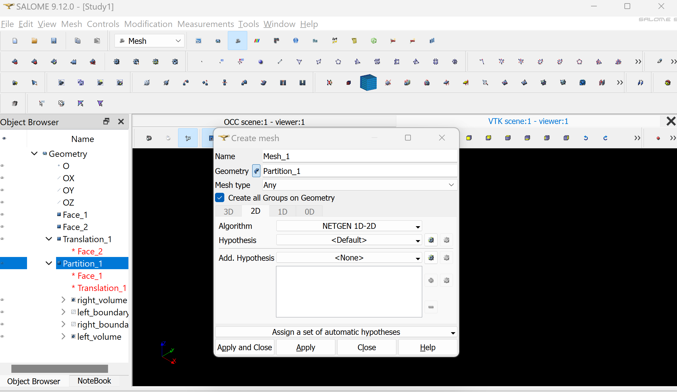
Next to “Hypothesis” click on the gear symbol. Select “NETGEN 2D Simple Parameters”. Click Ok. Click “Apply and Close”.
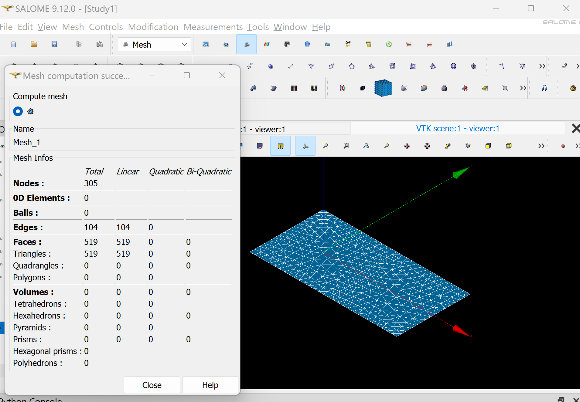
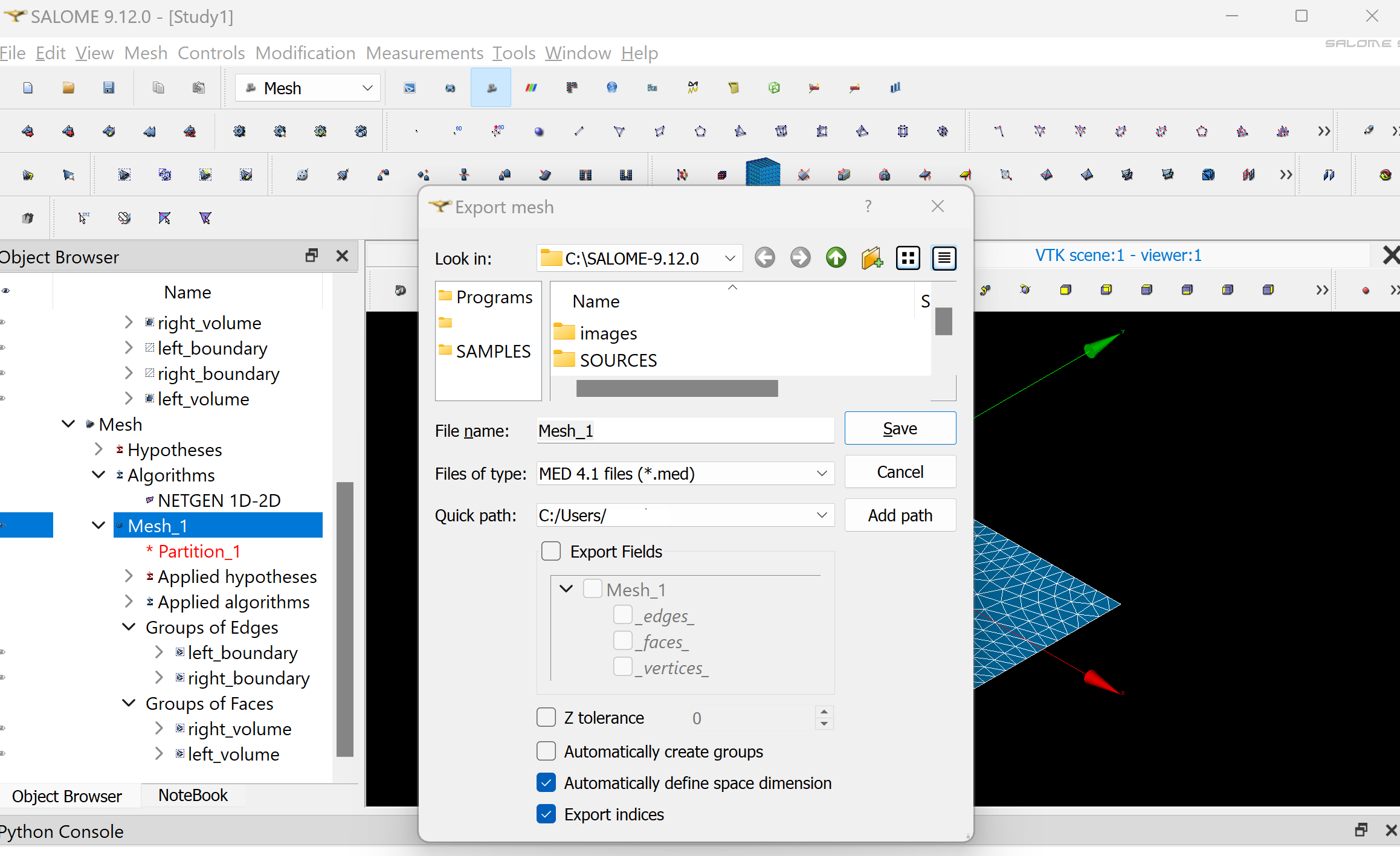
In the Objet Browser, under Mesh_1 you should see Groups of Edges and Groups of Faces, containing left_boundary, right_boundary, left_volume and right_volume.#
Export the mesh to MED by right clicking on Mesh_1 in the Object Browser, then Export/MED file. Choose a location where you want to write your MED file and click Save.
Convert mesh with meshio (at the time or writing we are using meshio 5.3)
python convert_mesh.py
The script convert_mesh.py is:
import meshio

def convert_med_to_xdmf(
    med_file,
    cell_file="mesh_domains.xdmf",
    facet_file="mesh_boundaries.xdmf",
    cell_type="tetra",
    facet_type="triangle",
):
    """Converts a MED mesh to XDMF
    Args:
        med_file (str): the name of the MED file
        cell_file (str, optional): the name of the file containing the
            volume markers. Defaults to "mesh_domains.xdmf".
        facet_file (str, optional): the name of the file containing the
            surface markers.. Defaults to "mesh_boundaries.xdmf".
        cell_type (str, optional): The topology of the cells. Defaults to "tetra".
        facet_type (str, optional): The topology of the facets. Defaults to "triangle".
    Returns:
        dict, dict: the correspondance dict, the cell types
    """
    msh = meshio.read(med_file)

    correspondance_dict = msh.cell_tags

    cell_data_types = msh.cell_data_dict["cell_tags"].keys()

    for mesh_block in msh.cells:
        if mesh_block.type == cell_type:

            meshio.write_points_cells(
                cell_file,
                msh.points,
                [mesh_block],
                cell_data={"f": [-1 * msh.cell_data_dict["cell_tags"][cell_type]]},
            )
        elif mesh_block.type == facet_type:
            meshio.write_points_cells(
                facet_file,
                msh.points,
                [mesh_block],
                cell_data={"f": [-1 * msh.cell_data_dict["cell_tags"][facet_type]]},
            )

    return correspondance_dict, cell_data_types


if __name__ == "__main__":
    filename = "Mesh_1.med"
    correspondance_dict, cell_data_types = convert_med_to_xdmf(
        filename, cell_type="triangle", facet_type="line")
    print(correspondance_dict)
Running this script produces mesh_domains.xdmf, mesh_boundaries.xdmf, mesh_domains.h5, mesh_boundaries.h5 and a dictionary of correspondance between the markers and the mesh entities:
{-6: ['left_volume'], -7: ['right_volume'], -8: ['left_boundary'], -9: ['right_boundary']}
The correspondance dictionary can be used to assign the correct markers to the mesh. Here, the left volume is tagged with ID 6, the right boundary is tagged with ID 9.
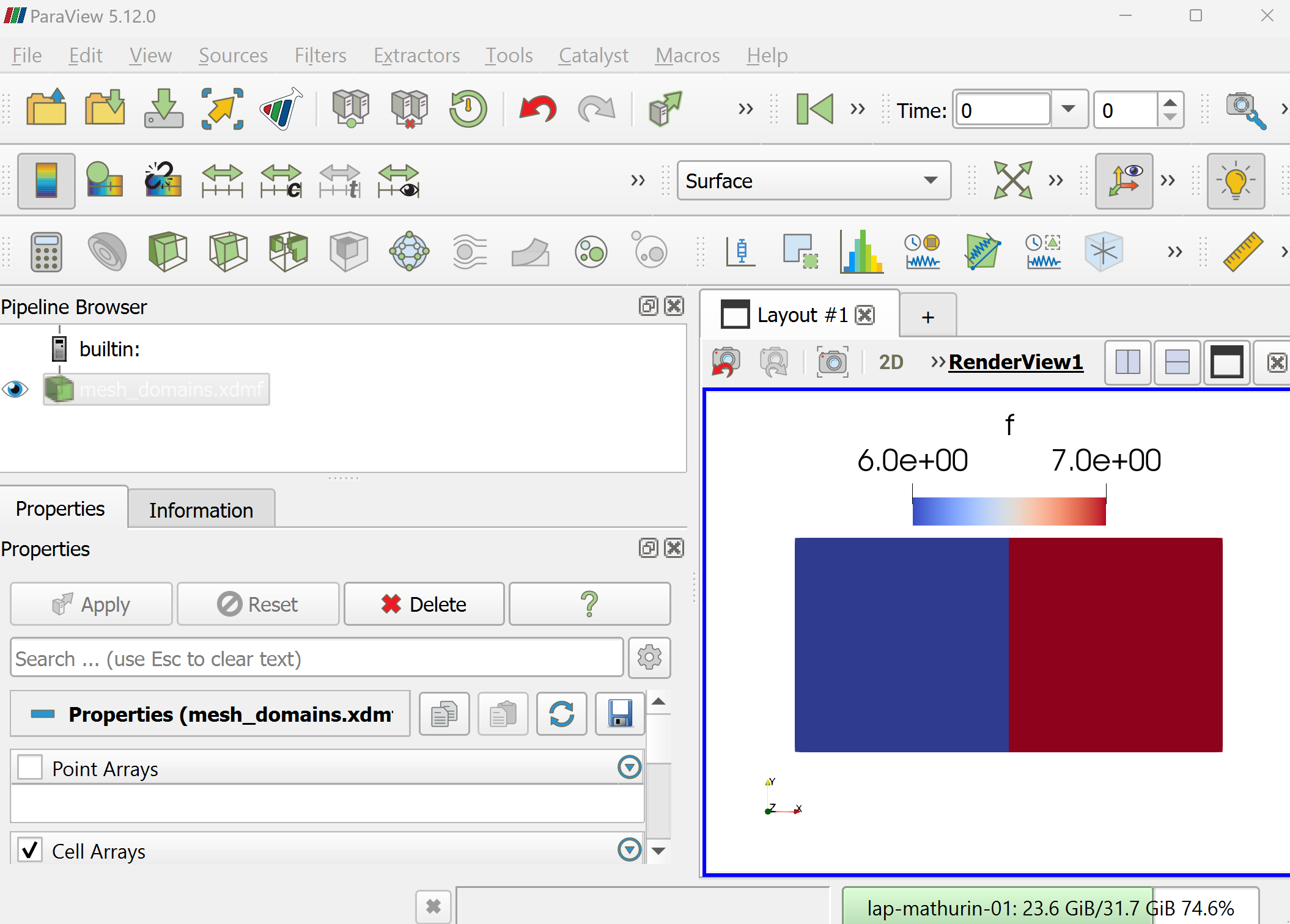
Inspect the produced XDMF files with Paraview using the XDMF3 S reader. The file mesh_domains.xdmf should look like:
Test the mesh in FESTIM by running:
import festim as F

model = F.Simulation()

model.mesh = F.MeshFromXDMF(
    volume_file="mesh_domains.xdmf", boundary_file="mesh_boundaries.xdmf"
)

model.materials = [F.Material(D_0=1, E_D=0, id=6), F.Material(D_0=5, E_D=0, id=7)]

model.boundary_conditions = [
    F.DirichletBC(field="solute", value=1, surfaces=[8]),
    F.DirichletBC(field="solute", value=0, surfaces=[9]),
]

model.T = F.Temperature(823)

model.exports = [F.XDMFExport("solute")]

model.settings = F.Settings(
    absolute_tolerance=1e-10,
    relative_tolerance=1e-10,
    transient=False,
)

model.initialise()
model.run()
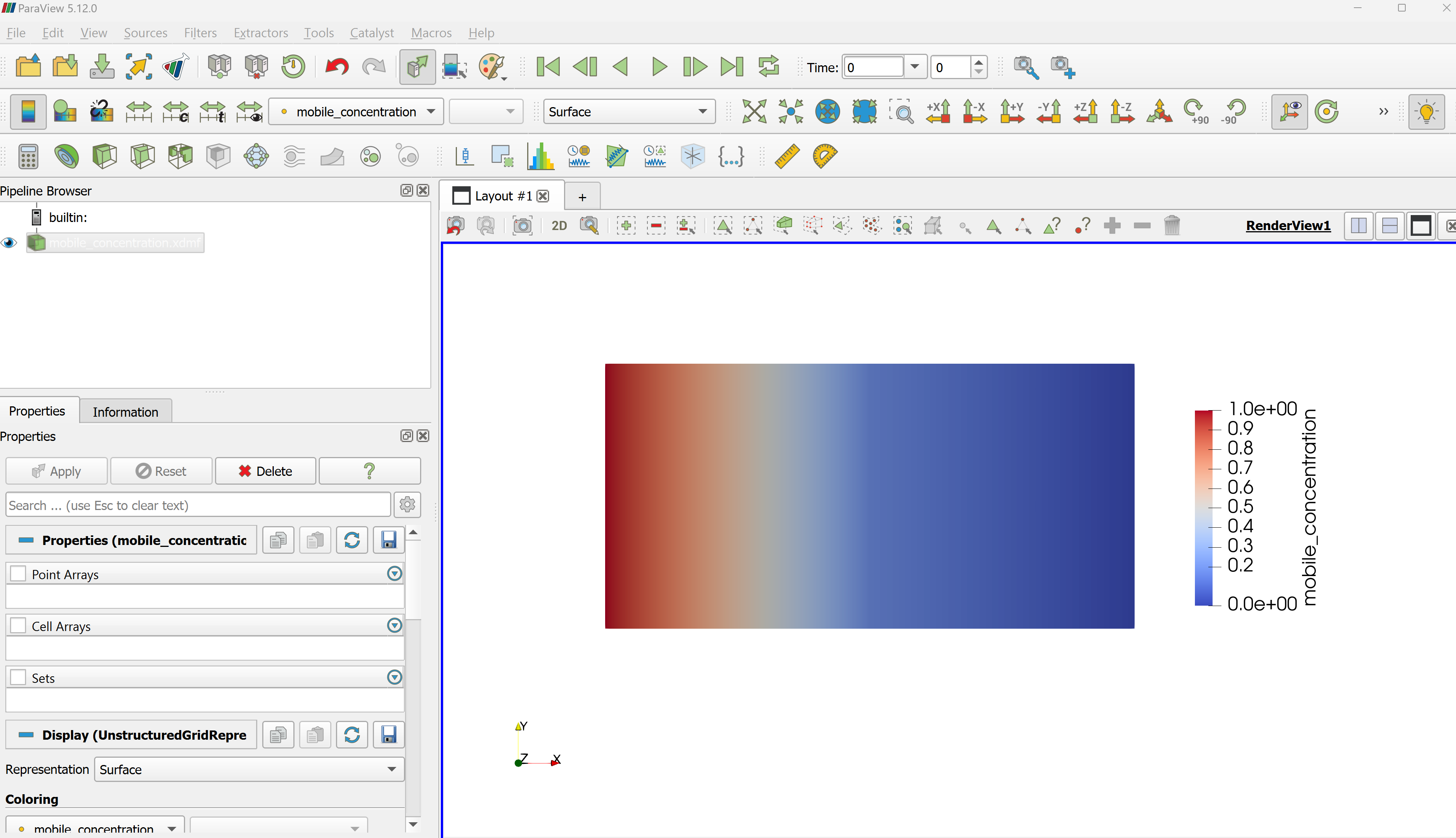
The simulation should run without errors. The solute field can be visualised with Paraview.
Meshing CAD files in SALOME#
If you have a CAD model, you can export it to a mesh with SALOME.
Create a new study
Activate the Geometry module
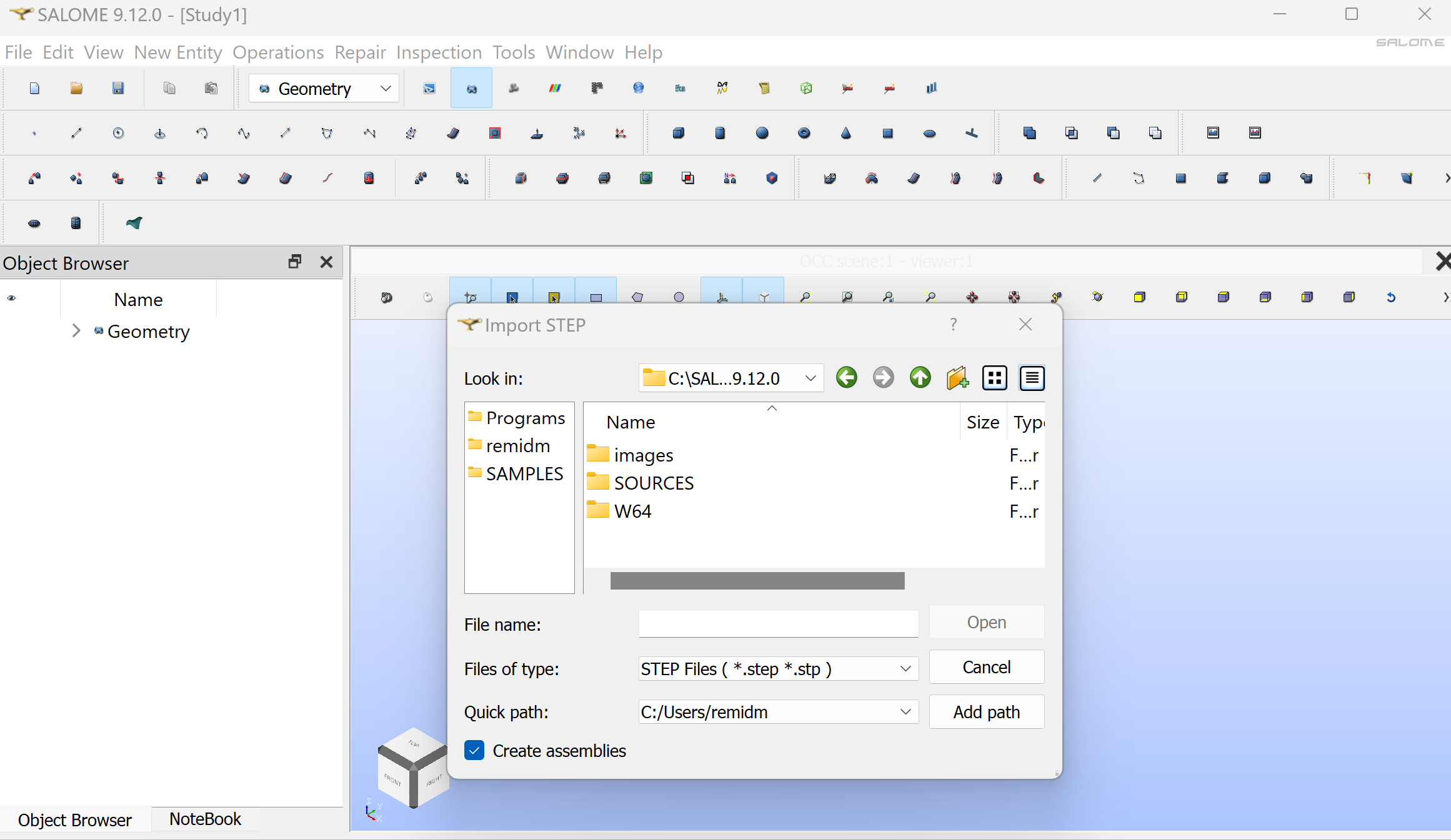
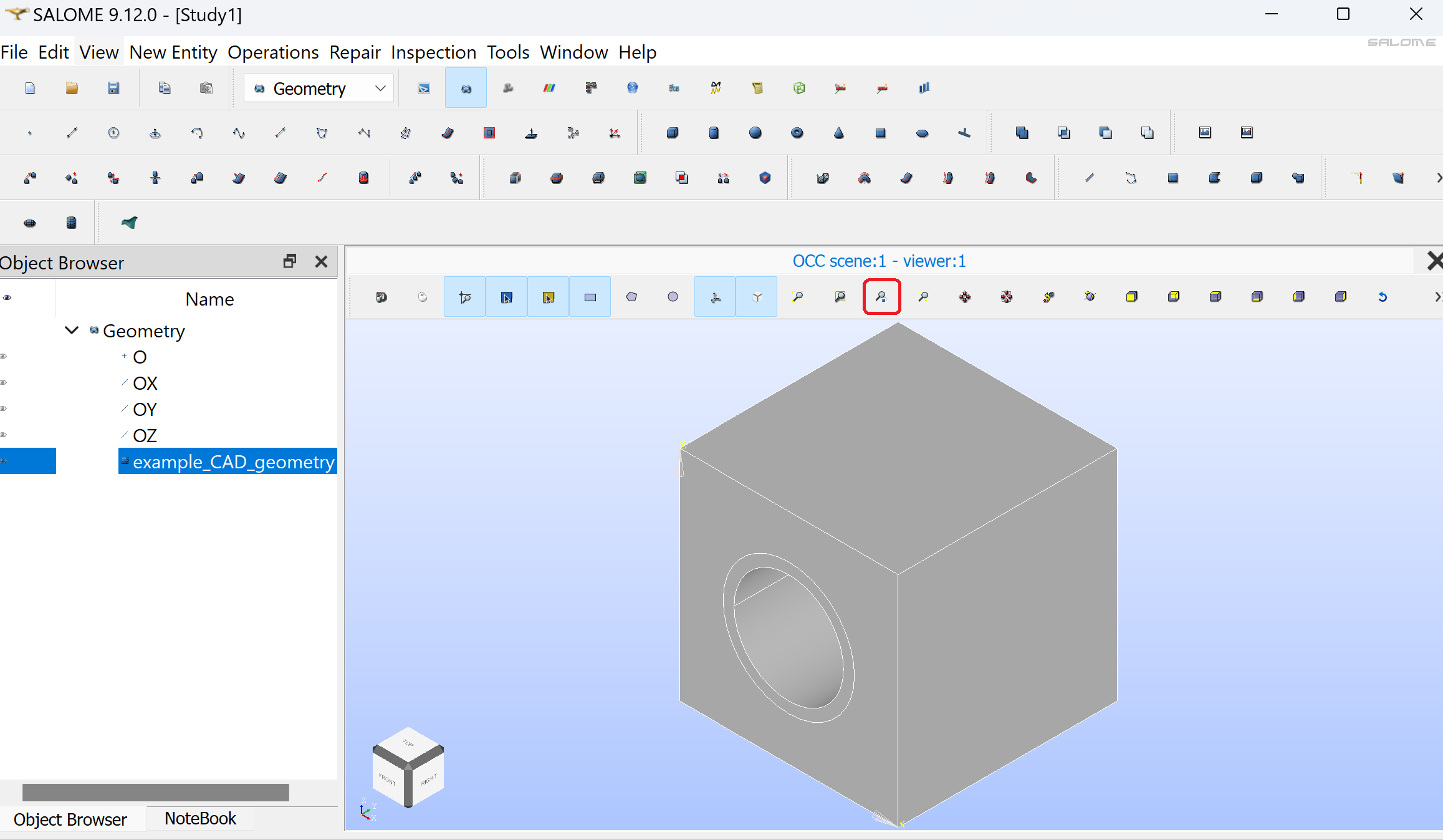
Import STEP file by clicking “File/Import/STEP”
By clicking “Fit to selection” you can see the imported geometry:
Create a partition just like in the previous example
Create groups of volumes and faces
Mesh the geometry
Export the mesh to MED
Convert the mesh to XDMF (don’t forget to change the cell and facet types in the script)
Meshes from FEniCS#
See the FEniCS documentation for more built-in meshes.