Post-processing#

Exports are added to the simulation object as a list of festim.Export objects:

import festim as F

my_model = F.Simulation()

my_model.exports = [..., ...]

Exporting solutions#

XDMF export#

The most straightforward way to export solutions (concentrations, temperature) with FESTIM is to use the festim.XDMFExport class. This class leverages the XDMFFile class of fenics and allows solutions to be exported in the XDMF format. The following example shows how to export the solution of a 1D problem:

import festim as F
import numpy as np

my_model = F.Simulation()
my_model.mesh = F.MeshFromVertices(np.linspace(0, 1, 60))
my_model.materials = F.Material(id=1, D_0=1, E_D=0)
my_model.boundary_conditions = [
    F.DirichletBC(surfaces=[1, 2], value=0, field="solute"),
]
my_model.sources = [F.Source(value=1, volume=1, field="solute")]

my_model.T = F.Temperature(500)

my_model.exports = [
    F.XDMFExport(
        "solute",  # the field we want to export
        label="mobile",  # how the field will be labelled in the XDMF file
        filename="./mobile_conc.xdmf",
        checkpoint=False,  # needed in 1D
    )
]

my_model.settings = F.Settings(
    absolute_tolerance=1e-10, relative_tolerance=1e-10, transient=False
)

my_model.initialise()
my_model.run()

Running this should produce two files called mobile_conc.xdmf and ˋmobile_conc.h5` in the current directory. The file can then be opened in Paraview or any other software that can read XDMF files. Here are some tips for using Paraview:

Make sure to have the h5 file in the same directory as the XDMF file
Do not modify the name of the files after their creation by FESTIM. This would result in not being able to open the file in paraview because the XDMF points to the h5 file
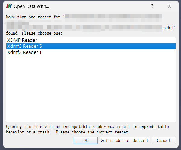
Open the XDMF file then select the reader Xdmf3 Reader S

Edit the colour map and rescale the colourbar to present the proper view of results

Find out more information on Paraview tutorials

For transient simulations, by default, festim.XDMFExport will export the solution at each timestep. It is possible to change this behaviour to limit the number of times the file is written to. By setting the mode attribute to 10, for example, the solution will be exported every 10 timesteps. Setting it to last will export the solution only at the last timestep.

my_model.exports = [
    F.XDMFExport(
        "solute",
        label="mobile",
        filename="./mobile_conc.xdmf",
        checkpoint=False,
        mode=10,
    )
]

The checkpoint attribute must be set to True for the XDMF file to be readable by Paraview.

TXT export (1D)#

The TXTExport class allows solutions to be exported in a simple text format. It works in 1D only. For multi-dimensional problems, use the festim.XDMFExport class instead.

import festim as F

my_export = F.TXTExport(field="solute", filename="./mobile_conc.txt")

Adding this export to the simulation object will produce a file called mobile_conc.txt in the current directory. This file will contain the solution of the solute field at the degrees of freedom of the mesh and at each timestep.

To only export at specific times in the simulation, use the times argument:

my_export = F.TXTExport(
    field="solute", filename="./mobile_conc.txt", times=[0, 1, 2, 3]
)

Point value#

If information about the solution at a specific point is needed, the festim.PointValue class can be used. It is implemented as a derived quantity. See Derived quantities for more information. Here are a few examples:

import festim as F

my_export = F.PointValue(field="solute", x=[0.5, 0.5, 0.5])
my_export = F.PointValue(field="solute", x=(0.5, 0.5, 0.5))
my_export = F.PointValue(field="solute", x=[0.5, 0.5])
my_export = F.PointValue(field="solute", x=[0.5])
my_export = F.PointValue(field="solute", x=0.5)

Derived quantities#

In addition to exporting the actual solutions, it is possible to export derived quantities. For instance, you may want to compute the flux of mobile particles at a given boundary.

First, you want to create a festim.DerivedQuantities object. This will encompass all the derived quantities you want to compute. Then, you can add the derived quantities you want to compute to this object. Finally, you can add the festim.DerivedQuantities object to the simulation object.

my_derived_quantities = F.DerivedQuantities(
    [
        F.SurfaceFlux(field="solute", surface=3),
        F.SurfaceFlux(field="T", surface=1),
        F.AverageVolume(field="retention", volume=1),
        F.TotalVolume(field="retention", volume=2),
    ]
)

my_model.exports = [my_derived_quantities]

The complete list of derived quantities can be found at: Exports.

Note

There is a specific derived quantity festim.AdsorbedHydrogen which can be used only with festim.SurfaceKinetics.

Accessing the data#

The data can be accessed in three different ways:

directly from the festim.DerivedQuantities (plural) object:

my_derived_quantities = F.DerivedQuantities(
    [
        F.SurfaceFlux(field="solute", surface=3),
        F.AverageVolume(field="T", volume=1),
        F.AverageVolume(field="retention", volume=1),
        F.TotalVolume(field="retention", volume=2),
    ]
)

my_model.exports = [my_derived_quantities]

my_model.initialise()
my_model.run()

print(my_derived_quantities.t)
print(my_derived_quantities.data)

from the festim.DerivedQuantity (singular) object (eg. F.SurfaceFlux(...)):

flux_surf_3 = F.SurfaceFlux(field="solute", surface=3)

my_derived_quantities = F.DerivedQuantities(
    [
        flux_surf_3,
        F.AverageVolume(field="T", volume=1),
        F.AverageVolume(field="retention", volume=1),
        F.TotalVolume(field="retention", volume=2),
    ]
)

my_model.exports = [my_derived_quantities]

my_model.initialise()
my_model.run()

print(flux_surf_3.t)
print(flux_surf_3.data)
print(my_derived_quantities[2].data)

In the previous case, we created a variable flux_surf_3 that is a festim.DerivedQuantity object. If this is not possible, the festim.DerivedQuantity object can be accessed with the festim.DerivedQuantities.filter() method:

my_derived_quantities = F.DerivedQuantities(
    [
        F.SurfaceFlux(field="solute", surface=3),
        F.AverageVolume(field="T", volume=1),
        F.AverageVolume(field="retention", volume=1),
        F.TotalVolume(field="retention", volume=2),
    ]
)

my_model.exports = [my_derived_quantities]

my_model.initialise()
my_model.run()

flux_surf_3 = my_derived_quantities.filter(fields="solute", surfaces=3)
print(flux_surf_3.data)

It is also possible to filter for several attributes values. For example:

total_vol = my_derived_quantities.filter(
    fields="retention",
    volumes=[1, 2],
    instances=F.TotalVolume,
    )

print(total_vol.data)

export and read from a .csv file:

my_derived_quantities = F.DerivedQuantities(
    [
        F.SurfaceFlux(field="solute", surface=3),
        F.AverageVolume(field="T", volume=1),
        F.AverageVolume(field="retention", volume=1),
        F.TotalVolume(field="retention", volume=2),
    ],
    filename="./my_derived_quantities.csv",
)

my_model.exports = [my_derived_quantities]

my_model.initialise()
my_model.run()

Compute and export every N timesteps#

By default, the derived quantities will be computed at each timestep and exported at the last timestep. This behaviour can be changed by setting the nb_iterations_between_compute and nb_iterations_between_exports attributes of the festim.DerivedQuantities object.

my_derived_quantities = F.DerivedQuantities(
    [
        F.SurfaceFlux(field="solute", surface=3),
        F.AverageVolume(field="T", volume=1),
        F.AverageVolume(field="retention", volume=1),
        F.TotalVolume(field="retention", volume=2),
    ],
    filename="./my_derived_quantities.csv",
    nb_iterations_between_compute=3,  # compute quantities every 3 timesteps
    nb_iterations_between_exports=10,  # export every 10 timesteps
)